Building a Vision-Only Chess Tracker
detecting chess moves from raw camera pixels on ordinary physical boards, across arbitrary board poses
Introduction: what is this about?
A chessboard forgets everything the moment you walk away - and that feels wrong.
I like chess, but I’m not a grandmaster. I play for fun, and I’m not too keen on memorizing opening lines or endgame traps.
My tech-avid, chess-playing brother wanted a simple way to track his real-life chess games. In this way he could analyze games offline to spot blunders, share the occasional masterpiece, maybe even track progress over time.
The concrete bet behind the project is simple: a normal camera should be enough. No RFID pieces, no magnetic board, no fixed top-down rig. Given two raw images of an ordinary physical board, the system calibrates the board pose, rectifies the camera view, compares the before/after pixels, and predicts the move that was just played.
Building such a system would be useful for:
- Offline analysis - capture the full chess game so computer engines and fellow players can dissect them long after the pieces are put away
- Progress tracking - a growing archive of your own moves lets you spot recurring mistakes and measure improvement over months, not just one session
- Hands-on ML playground - the project itself is a chance for both of us to build a practical computer-vision pipeline: real data, real constraints, and a clear success metric (did we log the right move?)
And of course use ✨ AI ✨ to do so. So of course, I said yes.
Chess Tracking: What is out there?
Chess Basics (for anyone who zoned out during The Queen’s Gambit)
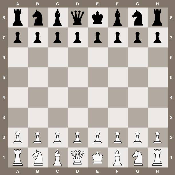
- Board – 8×8 grid = 64 squares, labelled a–h (files) and 1–8 (ranks). Two players, White and Black, face each other on opposite sides of the board. White moves first.
- Algebraic square names – bottom left from White’s view is a1, top right is h8.
- Universal Chess Interface (UCI) move format – four-char string: e2e4 = piece from e2 to e4; promotions add the piece letter (e7e8q).
- Pieces – king, queen, rook, bishop, knight, pawn (each with its own move pattern).
- Specials – castling (king+rook swap), en-passant capture, pawn promotion upon reaching the 8th rank.
- Goal – checkmate: king is attacked and can’t escape.
As always, ready-made solutions exist for this.
Commercial e-boards, like the DGT Smart Board, slot Hall-effect sensors beneath every square and rely on magnetized pieces to register moves [1].
Others, such as Chess Classics Exclusive or Chessnut Pro, embed an RFID chip in each piece and let an antenna grid read its identity and square in real time [2].
Both solutions hide the technologies under the squares or glue chips to every piece, making it quite pricey (€400+), fragile, and tied to one “smart” board.
We figured a minimal setup we already owned - basically a phone camera, a tripod, and a computer - should be enough to deal with this.
In short, we said “no, thanks” to sensor boards, because
- Extra hardware is awkward to carry around and takes effort to maintain/set up
- Most open places where you can play chess (parks, cafés, clubs) won’t ditch their own wooden sets / boards
- A decent camera lives in every pocket, so why not use it?
What makes camera-only tracking tricky
However, a camera-only approach comes with its own challenges, such as microscopic changes, move overload, real-world chaos, and timing the shots.
| Problem | Why it matters |
|---|---|
| Microscopic change | A single pawn moves forward; 95% of the pixels stay identical |
| Move overload | Dozens of legal moves can look almost the same in a still image |
| Real-world chaos | Shadows, glare, light changes, and the occasional elbow nudge to the board call for big misalignment and mispredictions. |
| Timing the shot | When to take a shot? the camera must fire after the piece lands but before the next hand enters |
As you will see, some of these issues are easy to solve with a bit of clever engineering, while others are more challenging and still bug us today. But let’s not get ahead of ourselves. Pull up a chair - we are about to make plain black-and-white images speak fluent chess.
As always, you can Check out the project on GitHub
Current project status. The repository is now packaged as a Poetry project under a standard
src/layout, with console-script entry points for dataset generation, training, prediction, the Flask API and the phone-camera demo. It also ships CI quality gates (ruff,ty,pytest) and a first tagged release,v0.2.0, which includes the companion Swing move recorder aschess-recorder.jar.
Our Journey towards a Vision-Only Chess Tracker
Before we could gloriously fail with neural networks, we needed a game plan. So we tried to decompose the problem into smaller pieces:
- Global goal: track the whole game → means keeping an accurate board state after every turn. Which means:
- Get board state after a turn = board state before + the move that just happened.
- Move detection → give the model two images (before / after) and ask, “Which square just emptied and which one just filled?”, basically obtaining the move in UCI format (e.g. e2e4, b7b8q, etc.).
- Move validation → even a clever model can hallucinate illegal jumps, so we must validate its guesses with a chess engine and keep only the legal moves in the current board state.
- State update → apply that validated move to our running board, then repeat from step 1 until handshake or checkmate.
- Get board state after a turn = board state before + the move that just happened.
Quick note: after all the above logic is implemented, we can simply record the taken moves and intermediate board positions into a standardized format (like PGN) and use it to analyze the game later on. This step is now handled by the companion Swing recorder attached to the latest GitHub release.
First Attempt: The SiameseNet
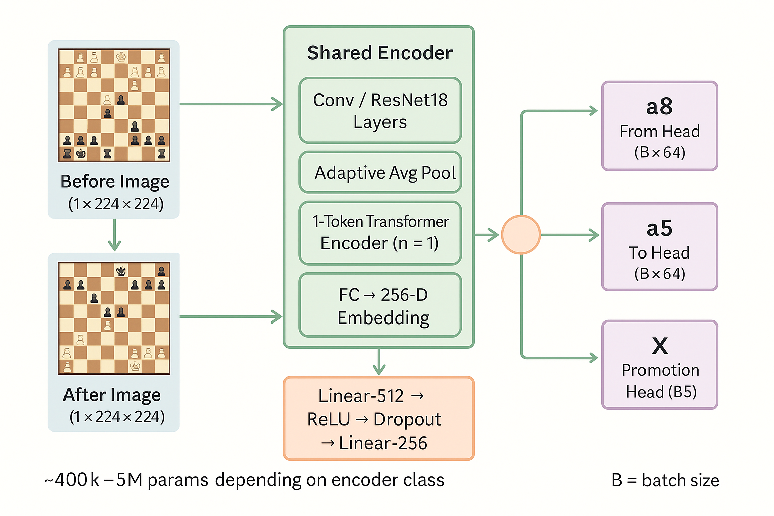
We started with a (possibly too) simple idea: shove the before and after move images through a single encoder network, concatenate the embeddings generated by the encoder together, and ask an MLP to predict the move in UCI format, i.e., from-square, to-square, and promotion. Such a double-headed model is called a Siamese network (SiameseNet for us).
You can see the diagram above for a simplified version of the SiameseNet pipeline. The code is still in the repository as the legacy image-pair baseline.
Here is a quick overview of our code:
# Example of a simple CNN encoder
class SmallCNNEncoder(nn.Module):
    def __init__(self, output_dim=256):
        super().__init__()
        self.encoder = nn.Sequential(
            nn.Conv2d(1, 16, kernel_size=5, stride=2, padding=2),  # -> [B, 16, 112, 112]
            nn.ReLU(),
            nn.MaxPool2d(2),  # -> [B, 16, 56, 56]
            ... # some more layers
            nn.AdaptiveAvgPool2d((1, 1)),  # -> [B, 64, 1, 1]
        )
        self.fc = nn.Linear(64, output_dim)

    def forward(self, x):
        x = self.encoder(x).view(x.size(0), -1)
        return self.fc(x)

# Actual move prediction model (SiameseNet)
class ChessMovePredictor(nn.Module):
    def __init__(
        self, embedding_dim=256, encoder_class: Type[nn.Module] = SmallCNNEncoder
    ):
        super().__init__()
        ...
        self.encoder = encoder_class(output_dim=embedding_dim)
        # MLP head
        self.mlp = nn.Sequential(
            nn.Linear(embedding_dim * 2, 512),
            nn.ReLU(),
            ...
        )
        # Output heads
        self.from_head = nn.Linear(256, 64)
        self.to_head = nn.Linear(256, 64)
        self.promotion_head = nn.Linear(256, 5)

    def forward(self, before, after):
        emb_before = self.encoder(before)  # [B, D]
        emb_after = self.encoder(after)  # [B, D]
        combined = torch.cat([emb_before, emb_after], dim=1)  # [B, 2D]
        x = self.mlp(combined)  # [B, 256]
        from_logits = self.from_head(x)  # [B, 64]
        to_logits = self.to_head(x)  # [B, 64]
        promotion_logits = self.promotion_head(x)  # [B, 5]
        return from_logits, to_logits, promotion_logits
For the encoder network, we tried different architectures, including our own Convolutional Neural Network (CNN), ResNet18 and Vision Transformers(ViT), but the first one was the most promising.
Data Generation process
In order to train the model, we needed a dataset of chess positions, with corresponding images, and annotations of the moves that were made. We generated a dataset of circa 20k chess positions, using the Blender rendering engine. The generation pipeline is as follows:
Step 1: Downloading and Analyzing Chess Games
We download chess games from Lichess. Our script fetches a large dataset of games and analyzes them to extract moves. We can specify the percentage of moves to retain and set a minimum count for each move type. The selected moves are shuffled and saved to a CSV file (entries.csv) for further processing.
For each move in the dataset, the script uses the FEN (Forsyth-Edwards Notation) strings to represent the board states before and after the move.
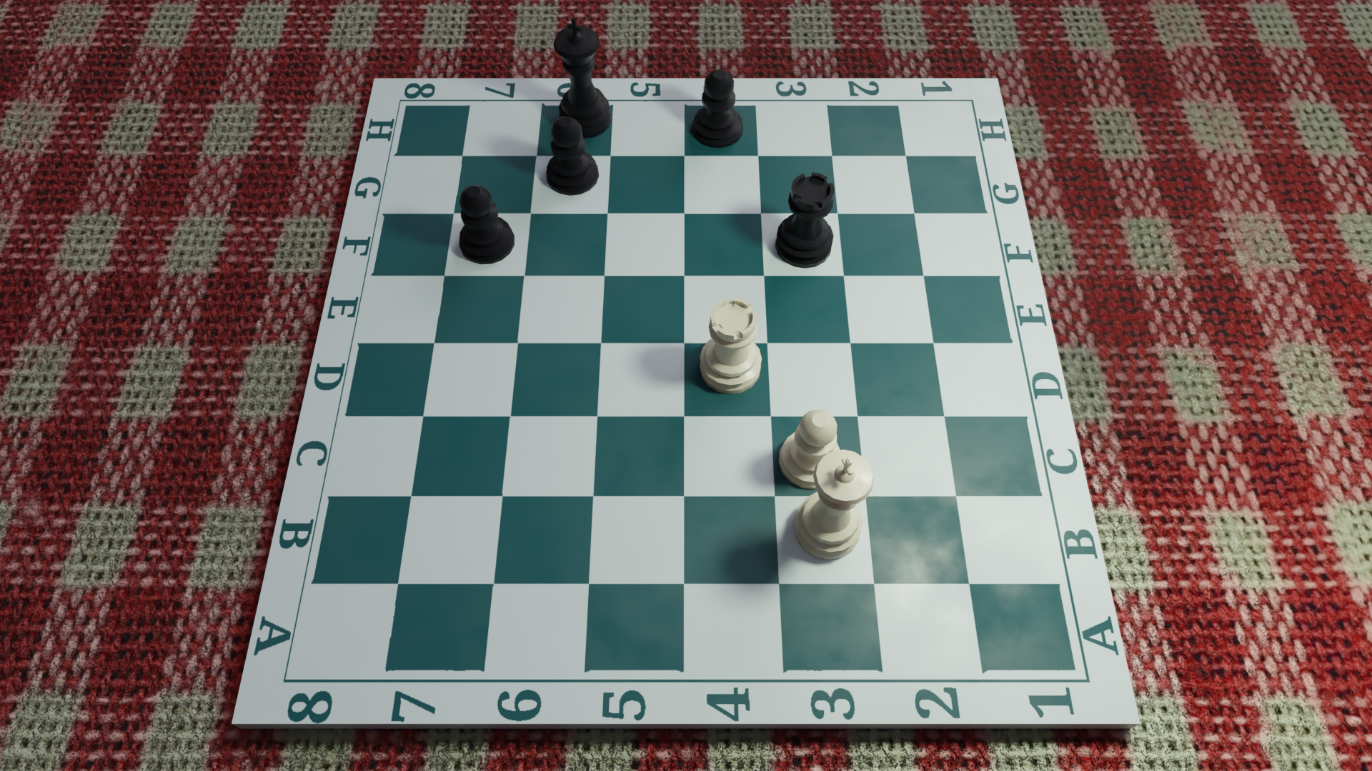
Step 2: Rendering Chess Move Configurations with Blender
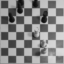
We use Blender to synthesize images of these board states in a tripod-realistic scenario (side shoot, 30-degree-ish angle downwards looking). We generate a variety of renders, differing in board look, piece style, and lighting conditions. This helps the model generalize better to different environments (see examples below).
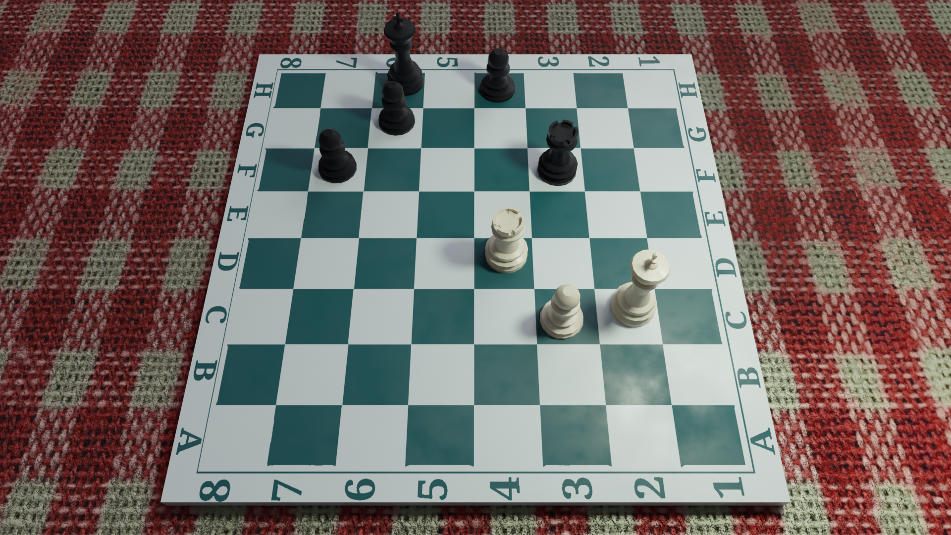
b3c2.
Finally, the board renders are pre-processed using OpenCV to rectify the perspective and normalize the images. The processed images are saved in the preprocessed directory. This is how the images look like after pre-processing:
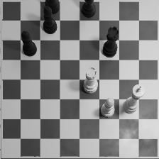
b3c2
Step 3: Dataset Preparation for Machine Learning
The generated images and move data are used to create PyTorch datasets. The first image-pair baseline used ChessMoveDatasetFromCSV, which loads preprocessed before/after images and labels them with move information (source square, target square, promotion). The current diff-patch model uses ChessMoveFromDiffDataset, which loads one diff image per move, splits it into 64 square patches, and returns the from/to labels used by the diff scorer.
class ChessMoveDatasetFromCSV(Dataset):
  ...
    def __getitem__(self, idx):
        before_tensor = self._load_image(before_id)
        after_tensor = self._load_image(after_id)
        label = {
            "from": torch.tensor(SQUARE_TO_IDX[from_sq], dtype=torch.long),
            "to": torch.tensor(SQUARE_TO_IDX[to_sq], dtype=torch.long),
            "promotion": torch.tensor(PROMOTION_TO_IDX.get(promo, 0), dtype=torch.long)
        }
        return before_tensor, after_tensor, label
Step 4: Training the Model
We train the first image-pair model using the generated dataset. As usual, we split the dataset into training and validation sets, and use the validation set to monitor the model’s performance during training. The legacy pair model is trained using a standard cross-entropy loss function (one for each predicting head), and we use an Adam optimizer with a fixed learning rate (1e-4) and a batch size of 32.
The training process involves feeding the model pairs of images (before and after the move) and their corresponding labels. The model learns to predict the move based on the visual changes between the two images.
Our First Experiments
What we monitored
We monitored the three following curves in our MLflow dashboard:
| Metric | Why we care |
|---|---|
| Training accuracy | Are we actually learning? |
| Validation loss | Early warning for overfitting |
| Validation accuracy | Top-1 hit rate on the synthetic hold-out set. |
So, what happened?
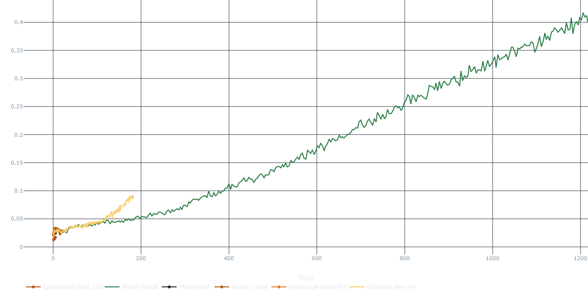
from and to heads of the model, over three different runs. As you can see, the model learns to predict moves from the training set with a fairly good accuracy (>35% each, over dozens of possibly illegal moves).
However, our network simply couldn’t generalize to the task. We tried different architectures, hyperparameters, and training strategies, but the model would still overfit the training set. We also figured it could be due to exceeding model capacity - so we reduced the number of parameters and tried again, but the results were still disappointing.
This led us to rethink the approach. We came up with three main reasons why the model was failing:
- Global features drown tiny changes – ResNet focuses on fine-grained patterns (blobs, edge); but cell-shifted pieces hardly relate to these patterns
- 20k renders are small for a full-image model – easy to overfit on board textures and camera angle.
- Too difficult to satisfy – the MLP had to learn piece legality and visual change in one shot.
Our key takeaway: we should detect the change, not the pieces or the board.
We realized the network should focus only on what was moved, we ditched the Siamese idea and moved toward our diff-patch pipeline - the one you’ll meet in the next section.
(Yes, the Blender pipeline we used to create those 20k boards almost stayed the same.
We’ll revisit data synthesis in the sections below.)
The Aha! Moment – Go Small, Go Local, Go Δ
“RIP SiameseNet (2025-2025) ✝️”
Suddenly, we had a realization moment: a legal move usually changes two squares: one goes empty, one gets a new piece. So instead of letting a big CNN stare at the whole board, we could apply a magnifying glass over every square and ask, “Did you change?” It’s like running 64 tiny analyses rather than one blurry wide-angle shot.
But in order for this to work, cells need to be comparable across images. So we needed to make sure that the images were aligned and that the pieces were in the same position in both images.
This is where the homography comes in. We use OpenCV to detect the board corners from calibration images and compute a perspective transform from the camera view to a normalized top-down board crop. This gives us comparable square coordinates even when the camera sees the board from an oblique pose.
In short, the new pipeline looks like this:
- Offline calibration – use OpenCV to recover the board corners and the homography from camera pixels to a normalized board plane.
- Capture before / after frames – take a picture of the board before and after the move.
- Pre-process – warp the images using the homography matrix, convert to grayscale, and normalize.
- Diff – compute the absolute difference between the two images and normalize it.
- Slice into 64 patches – crop the diff image into 64 patches, one for each square on the board.
- PatchEncoder – apply a small CNN to each patch to extract features.
- MoveScorer – compute a similarity score between the patches to predict the move.
- Legality filter – use a chess engine (like python-chess) to check if the predicted move is legal.
- Output – if the move is legal, update the board state and continue to the next turn.
- Save the game – save the moves and board state to a PGN file for later analysis.
- Repeat – go back to step 2 until the game is over.
Note: this is not _entirely_ true, as some moves can involve more than two squares (e.g. castling, en-passant, and promotions). However, these cases are rare and can be handled separately.
Step 1: Adapt Our Data Generation Pipeline
We add one more step at the end of the data generation pipeline, to standardize images across poses and compute difference between before and after frames.
diff_img = cv.absdiff(before_img, after_img)

if binary:
    _, diff_img_binary = cv.threshold(diff_img, binary_threshold, 255, cv.THRESH_BINARY)
    return diff_img_binary
else:
    return diff_img
In this way we generate standardized diff images that highlight the changes between the “before” and “after” board states. These images are saved in the diff directory and can be used for tasks like move prediction or board state classification.
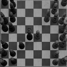
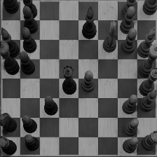
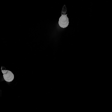
c8g4 (before, after, and diff images).
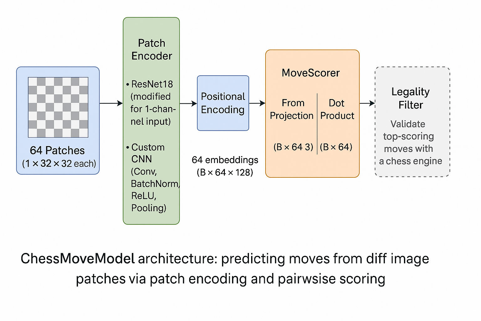
Step 2: Adapt Our Model
We ditched the Siamese network and moved to a new architecture, which we call PatchEncoder. This model has two key differences: 1) focuses on the differences between the two images, by applying a small CNN directly to the diff image, 2) operates on patches, i.e. cell-wise crops of the diff image, which contain the pixels of a single square.
The new PatchEncoder model takes the diff image as input (cropped into 64 patches) and applies a series of convolutional layers to extract features. The output is a set of embeddings for each patch, which are then used to predict the move.
The current implementation lives in src/chess_detector/models/diff.py, and the corresponding training entry point is src/chess_detector/training/train_diff.py.
Here is the rough code for the PatchEncoder model:
class ConvPatchEncoder(nn.Module):
    def __init__(self, in_channels=1, embed_dim=128):
        super().__init__()
        self.cnn = nn.Sequential(
            nn.Conv2d(in_channels, 32, kernel_size=3, padding=1),  # [B, 32, 32, 32]
            nn.BatchNorm2d(32),
            nn.ReLU(),
            nn.MaxPool2d(2),  # [B, 32, 16, 16]
            nn.Conv2d(32, 64, kernel_size=3, padding=1),  # [B, 64, 16, 16]
            ... # many more layers
            nn.ReLU(),
            nn.MaxPool2d(2),  # [B, 128, 4, 4]
        )

        # Final projection to embed_dim
        self.fc = nn.Linear(128 * 4 * 4, embed_dim)

    def forward(self, patches: torch.Tensor) -> torch.Tensor:
        B, N, C, H, W = patches.shape
        patches = patches.view(B * N, C, H, W)  # [B*64, 1, 32, 32]
        features = self.cnn(patches)  # [B*64, 128, 4, 4]
        features = features.view(B * N, -1)  # [B*64, 2048]
        embeddings = self.fc(features)  # [B*64, embed_dim]
        embeddings = embeddings.view(B, N, -1)  # [B, 64, embed_dim]
        return embeddings
This forces the model to focus on learning whether a square was involved in the move or not, rather than trying to learn the whole board state.
Step 3: Adapt our Move Predictor
We also changed the way we compute the final move. In our new MoveScorer model, we use an attention-like mechanism to compute the relationship between the 64 cells of the board. The model takes the 64 cell embeddings from the PatchEncoder and
1) adds positional encodings to each patch to retain spatial information
2) computes two linear projections of the embeddings: one for the from square and one for the to square. This enforces the model to learn the relationship between the patches and the move.
3) computes a dot product similarity score between the from and to projections, which is then interpreted as the move score. These dot-product logits are scaled by a learned temperature parameter to control the sharpness of the distribution.
This is the rough implementation of the MoveScorer model:
class MoveScorer(nn.Module):
    def __init__(self, embed_dim=128, proj_size=32):
        super().__init__()
        self.from_proj = nn.Linear(embed_dim, proj_size)
        self.to_proj = nn.Linear(embed_dim, proj_size)
        self.temperature = nn.Parameter(torch.tensor(1.0))

    def forward(self, embeddings: torch.Tensor) -> torch.Tensor:
        # embeddings: [B, 64, embed_dim]
        from_vecs = self.from_proj(embeddings)  # [B, 64, proj_size]
        to_vecs = self.to_proj(embeddings)  # [B, 64, proj_size]

        # Compute pairwise move scores using batched matrix multiplication and
        # normalize by learned temperature
        scores = (
            torch.matmul(from_vecs, to_vecs.transpose(1, 2)) * self.temperature
        )  # [B, 64, 64]
        return scores
Putting all together, the new model architecture looks like this:
class ChessMoveModel(nn.Module):
    def __init__(
        self,
        patch_size=32,
        in_channels=1,
        embed_dim=128,
    ):
        super().__init__()
        self.encoder = ConvPatchEncoder(in_channels=in_channels, embed_dim=embed_dim)
        self.scorer = MoveScorer(embed_dim=embed_dim)
        self.positional_encoding = nn.Parameter(torch.randn(64, embed_dim))

    def forward(self, patches: torch.Tensor) -> torch.Tensor:
        # patches: [B, 64, C, H, W]
        embeddings = self.encoder(patches)  # [B, 64, embed_dim]
        embeddings = embeddings + self.positional_encoding.unsqueeze(0)  # [B, 64, embed_dim]
        scores = self.scorer(embeddings)  # [B, 64, 64]
        return scores
The final move prediction scores of shape [64 x 64] (from-to pairs) are then passed to a legality filter (using python-chess) to find the first legal move (in decreasing order of likelihood). Given this move, we can update the board state and continue to the next turn.
Training & Results — the Diff-Patch Network In the Wild
In addition to the three metrics we tracked in the previous section, we added one more to help us understand how the model is performing:
| Avg. GT-move score | Mean softmax score assigned to the correct move - tells us how confident the model is even when it’s right. |
(Each colored line is one training run with a different hyperparam config; the funky MLflow names stayed in.)
What the curves say
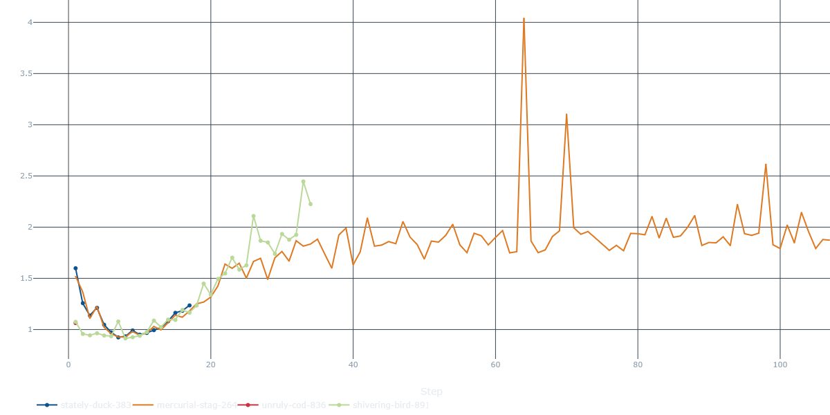
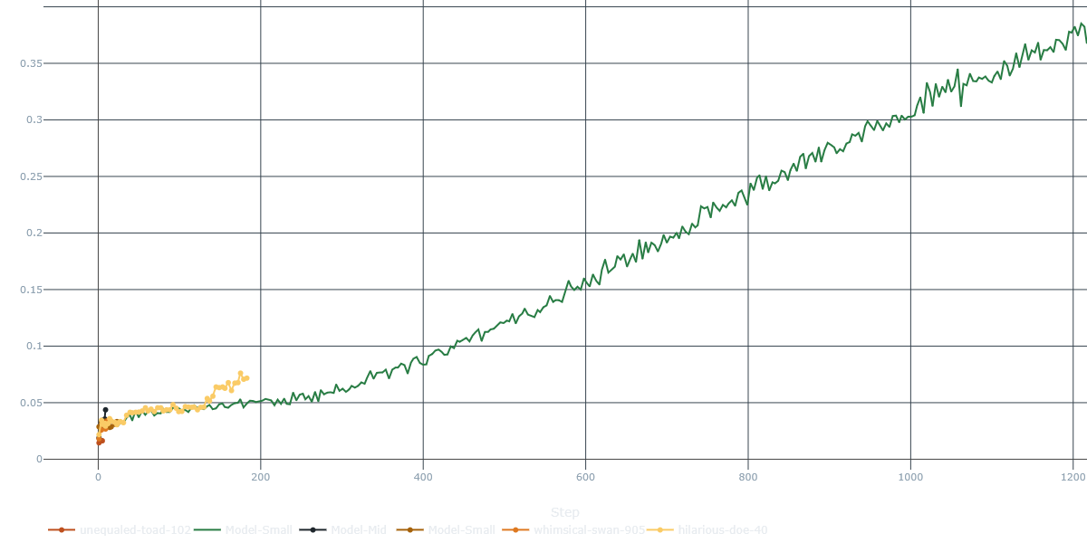
MoveScorer)- Text-book convergence, with U-shape = over-fit. Validation cross-entropy free-falls from 2.x to <0.9 in 10 steps, then creeps up.
- The orange run occasionally spikes above 3.5 — we traced those to learning-rate bursts; easy fix with a milder schedule.
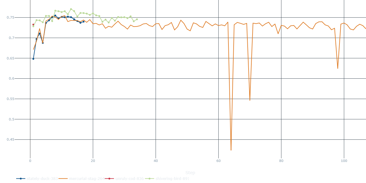
MoveScorer)- Rapid climb, early plateau. All runs surge from ≈0.45 → 0.65 in the first 10 steps, then level around 0.71 – 0.73.
- The best run (blue) keeps nudging upward, flirting with 0.77 by step 10.
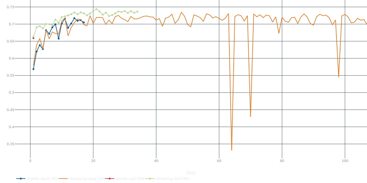
MoveScorer)- Confidence rises with accuracy: GT-move prob climbs from 0.58 → 0.74 and stays there.
-
Orange run again shows confidence dips that match the loss spikes.
-
An alternative logging confirms a ~0.77 top-1 and a 0.95 top-2 ceiling for the most stable seed - not bad at all for a 650k-param network.
- We also evaluated the model on a small set of real-world images (taken with a smartphone camera) and achieved around 60% accuracy on the first try.
TL;DR performance
| Dataset | Top-1 | Top-2 | Note |
|---|---|---|---|
| Synthetic validation (20k positions) | 0.77 | 0.95 | After 30 training steps, before over-fit kicks in |
Other Observations
- Fast learning: most of the lift happens in <15 minutes on a Nvidia RTX 3090.
- Early-stop sweet-spot: stepping out around epoch 30 captures peak val-acc and lowest val-loss.
Outcome? A 650k-param network (617k for the encoder alone) that nails ¾ of synthetic moves in one shot on synthetic boards and still lands around 60% on first-try real photos.
Next steps: bigger real dataset, hardcore augmentation, and that long-promised promotion handling in the diff pipeline.
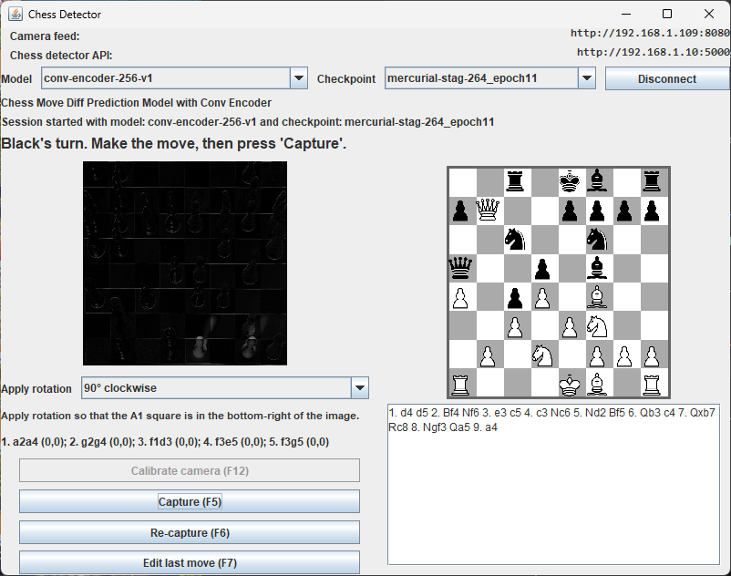
Putting It All Together: Create a User-Friendly Chess Tracker App
Having the model work with good accuracy is great, but we also need to make it user-friendly and easy to use. In particular, we need to make sure that the app can be used in real-time, with minimal setup and configuration.
Today the repository exposes two user-facing surfaces around that idea:
- a Tkinter phone-camera demo (
chess-detector-demo-phone) that pulls snapshots from an IP camera and talks to the Python prediction pipeline; - a companion Java Swing recorder, published as
chess-recorder.jaron the GitHub Releases page, for recording annotated moves from a physical-board session.
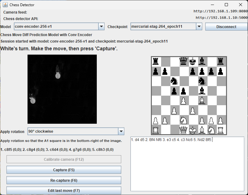
We create a simple GUI app with Java Swing that allows the user to:
- calibrate the board (get the corners of the chessboard)
- record a move (take a picture of the board before and after the move)
- display the predicted move
- display the current board state
- save the game to a PGN file
The main components of the app are:
-
Tripod – a simple tripod to hold the smartphone camera in place. The camera should be positioned above the board, with a clear view of all squares. We typically apply it on the left side, point at about 60 degrees angle down and at few centimeters from the board.
-
Camera – use a smartphone with an IP camera app (for example Android IP Webcam) to expose snapshots to the computer. The demo captures frames from the camera URL and processes them move-by-move.
-
Computer – a laptop or desktop computer running the app. The Python demo and Flask API are shipped as separate console scripts, while the Swing recorder focuses on calibration, move capture, board-state display and PGN export.
Strengths, Weaknesses & Next Steps
✔ Strengths
- Works on any board, any pieces, no fancy RFID or magnets required
- Zero extra hardware – just your phone cam, a tripod, and a laptop
✘ Weaknesses
- Finicky lighting or a tiny tripod bump can scramble the diff image
- Pawn promotions? Still on our TODO list (sorry, under-appreciated queens)
On our Roadmap
- Bigger real-world dataset – parks, clubs, dodgy basement lighting
- Aggressive augmentation – glare jitter, motion blur, piece style swaps
- Dual-exposure trick – snap twice, merge for better low-light diff maps
- Promotion-head revival – give pawns their rightful upgrade path
- Online board tracker – continual pose re-calibration to shrug off nudges
Fun-Size Takeaways
- Synthetic > manual - Blender renders beat hours of hand-labeling of real images
- Pose first, pixels second - recover the board plane before asking the model what changed
- Zoom then learn - focus on the changed squares and even tiny CNNs can shine
- Simple beats slick - two photos + clever math trump sensor-stuffed boards
Sensors? Nah. We’re running this game on raw RGB.
Big thanks to Lorenzo Notaro for being my companion on this project, his help with the Blender pipeline and support in the long brainstorming and debugging sessions (besides, you have a better GPU than I have).
References
[1] DGT Electronic Chess Boards overview – chesshouse.com – https://www.chesshouse.com/collections/dgt-electronic-chess-boards-pc-connect
[2] Chessnut Pro sensor discussion – chessbazaar.com – https://www.chessbazaar.com/blog/enhancing-your-chess-experience-with-custom-chess-sets-from-chessbazaar-dgt-sensors-and-chessnut-pro-sensors/