What Should the Elevator Do?
Where RL Meets the Real World - and Gets Stuck Between Floors
Introduction: Elevators of the World, Unite 🚀
Have you ever wondered how elevators work?
Not in a strictly mechanical sense, but rather on an intelligence abstraction layer. Like, how do they decide where to go next?
This seemingly simple question opens the door (🚪 pun intended) to a surprisingly rich and nuanced problem.

Should elevators prioritize minimizing user wait times? Or aim for energy efficiency by reducing travel distance? Should they serve requests in the order they arrive, or optimize for overall throughput? And what happens when there’s more than one elevator in the building?
As passengers, we mostly care about convenience: how long we wait and how fast we reach our floor. But from the perspective of a building operator or engineer, different concerns emerge: how can we reduce energy use? Can we minimize wear and tear by limiting unnecessary stops or idle travel? How do we prevent overloads, ensure fairness, or avoid congestion during peak hours?
Both perspectives—human and operational—feed into what ultimately becomes the elevator’s control policy. It’s a deceptively complex decision space, filled with competing goals and evolving constraints.
To be clear, this isn’t a problem that keeps elevator manufacturers up at night. Real-world solutions are robust, often hardcoded, and backed by decades of engineering know-how. But from a simulation and AI perspective, it’s a beautiful sandbox: tractable yet non-trivial, bounded yet open-ended.
Bonus: The elevator problem maps one-to-one with the hard drive scheduling problem, where a disk head must serve read/write requests while moving across sectors—just like our elevator across floors. The similarity is so strong that the SCAN disk algorithm is literally nicknamed “the elevator algorithm.”
Apparently, I’m not the only one intrigued by this:
- Elevator Saga game: program your own elevator logic.
- Reddit challenge: an elevator problem in code.
- Discussion thread: elevator scheduling gets nerdy.
So why not simulate it? In this post, I’ll walk you through building a simple elevator simulator in Python, complete with classical and reinforcement learning agents. We’ll explore how to model the problem, set up the environment, and train an RL agent to learn optimal elevator dispatching strategies.
Background: How Do Real Elevators Work?
Before diving into simulations and algorithms, it’s worth understanding how real elevators make decisions. At first glance, an elevator seems simple: press a button, wait, ride, done. But beneath that simplicity lies a surprisingly thoughtful logic.
Elevator systems process two types of external requests, known as hall calls:
- Up requests — triggered when a user presses the “Up” button on a floor
- Down requests — triggered when the “Down” button is pressed
Once inside the cabin, users input their destination floor — these are called car calls.
The elevator controller maintains a list of these requests and decides where the elevator should go next, and in what order.
Collective Control: Real-World SCAN in Action 🚦
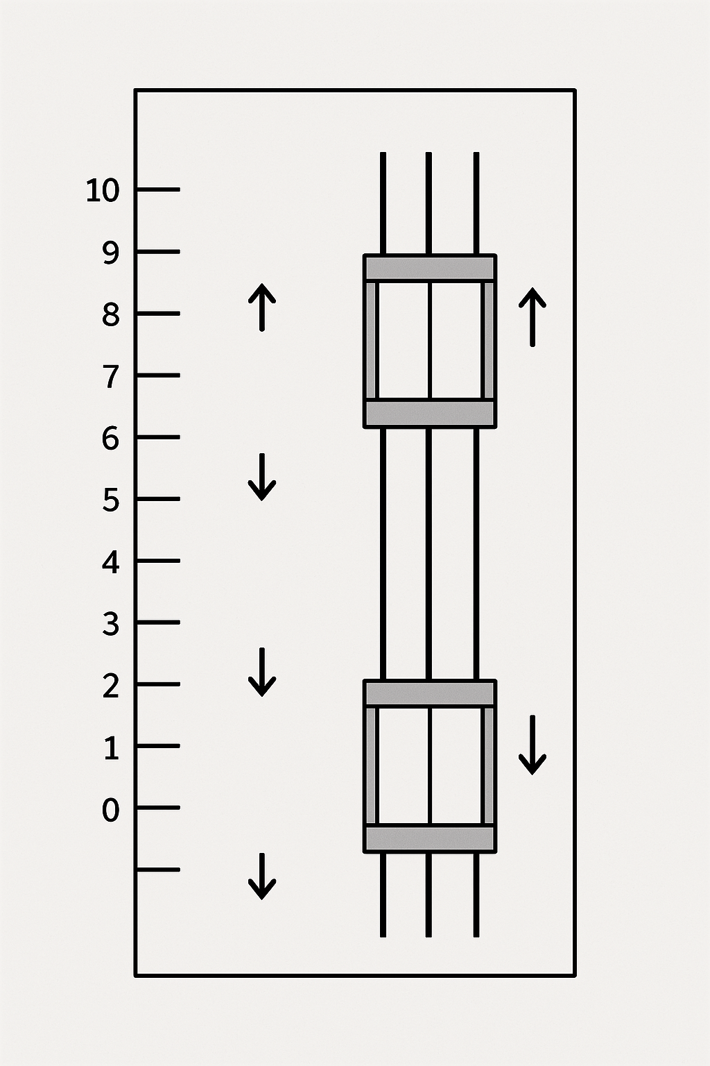
Most commercial elevators use a rule-based strategy called collective control1. In this approach, the elevator picks a direction (up or down) and serves all outstanding requests in that direction — both hall and car calls — before reversing.
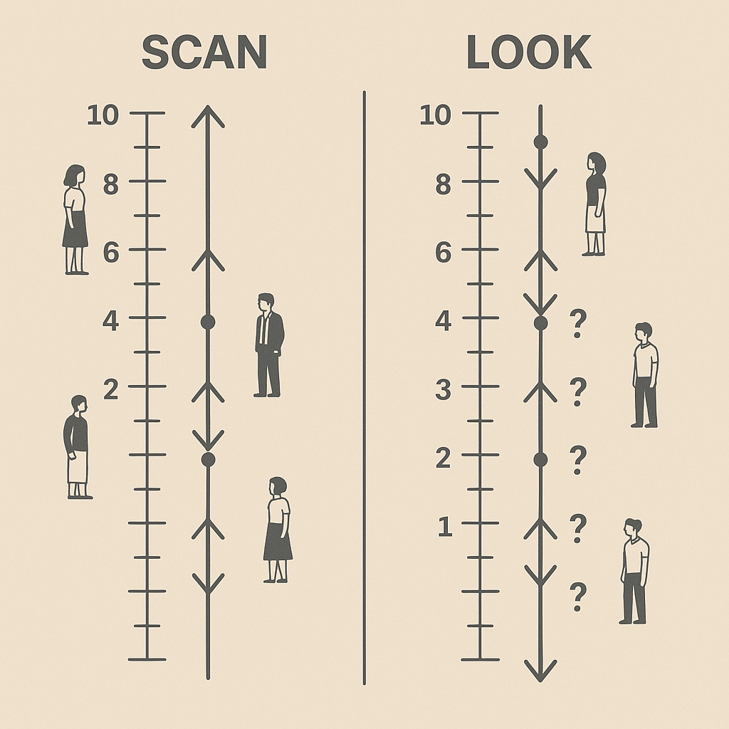
This behavior directly mirrors the classical SCAN algorithm2, also known as the “elevator algorithm” in disk scheduling. SCAN moves sequentially in one direction, handling requests along the way, and reverses only when it reaches the furthest request (or edge). Collective control works the same way: the elevator sweeps up, serving all upward requests, then sweeps down for downward ones.
The advantage? It avoids starvation (no request waits forever) and reduces unnecessary direction changes.
Dynamic Look-Ahead: Enter LOOK Behavior 👀
Some elevators implement a more refined strategy: instead of always going to the top or bottom floor, they turn around at the last requested stop in the current direction. This is the LOOK algorithm, a variant of SCAN that stops short if there are no requests beyond a certain point.
For instance, if an elevator is going up and there are no requests above floor 8, it may reverse at 8 instead of going all the way to the top. This reduces empty travel and saves time, especially during light traffic.
Real-World Enhancements and Dispatching
In multi-elevator systems, another layer of decision-making is required: which elevator should respond to a hall call? Common strategies include:
- Nearest-Car (or Nearest-Request)3: assign the elevator closest to the call
- Coincidence Bonus: favor elevators that already plan to stop at the same floor
- Zoning1: elevators are assigned to serve specific floor ranges, minimizing overlap
- Traffic Modes: systems adapt based on time of day, e.g. morning up-peak prioritizes rapid returns to the lobby
Some modern elevators even use destination dispatch4, where passengers select their floor in the lobby, and are grouped into elevators heading to similar destinations. This can dramatically reduce the number of stops per trip, but these systems are more complex and require advanced algorithms to manage.
For the time being, we will focus on the simpler single-elevator case, where the elevator is responsible for serving all requests in a building.
Classical Scheduling Algorithms 🧮
To understand how elevators decide their next move, we can draw direct inspiration from classical disk scheduling algorithms.
-
First-Come, First-Served (FCFS): Requests are handled strictly in arrival order. It’s simple but inefficient for elevators, often leading to long detours.
-
SCAN (Elevator Algorithm): The elevator moves in one direction serving all requests, then reverses. This is the default for most elevators and mirrors collective control. It’s fair and avoids starvation, but may cause unnecessary travel to the top/bottom.
-
LOOK: Like SCAN, but turns around at the last request in the current direction—reducing unnecessary movement. It’s more efficient in scenarios with sparse or bursty requests.
Other notable strategies exists 5 such as SECTOR, Dynamic Loading Balancing (DLB), High Unanswered Floor First (HUFF) and many more.
These algorithms offer a foundation—but they struggle when requests become unpredictable, the system scales up, or multiple elevators must coordinate 6. Which brings us to…
So Why Not Use a Reinforcement Learning Agent? 🤖
What is RL?
Reinforcement Learning (RL) is a group of Machine Learning techniques focused on solving complex problems by interaction. An agent observes the environment, takes actions (like moving or stopping), and receives rewards based on the outcome (e.g., minimizing wait time). Over time, it learns to maximize cumulative reward through trial and error.
In our case, the agent isn’t just figuring out how to move, it’s learning why, when, and for whom. It can develop nuanced strategies like skipping unnecessary stops, idling near busy floors, or serving longer-waiting passengers first.
Why RL Sounds Great
- Model-free discovery: No need for complex rules or handcrafted heuristics—RL learns what works through interaction.
- Emergent behavior: even in data-scarce, single-elevator environment, RL can outsmart static algorithms like LOOK by:
- Skipping low-value stops, e.g. when the elevator is full or the detour is inefficient
- Prioritizing older requests (RL can learn to avoid starvation by giving priority to older calls)
- Breaking strict directionality , e.g. reverse or zigzag when it’s more efficient to do so
- Learning floor usage patterns, like always returning to the lobby during idle times
- Optimizing long-Term outcomes: Unlike greedy strategies, RL sees beyond the next stop—factoring in future rewards.
- It’s fun: Watching an agent figure out strategies is inherently satisfying for us tech nerds 😄
Why RL Is Tricky
- Training is expensive6: A heuristic runs in seconds. RL might need thousands of episodes to converge. Not cool.
- Reward Design is critical: A poorly crafted reward leads to nonsense behavior or diverging training.
- Local Optima: The agent may learn odd behaviors (like “jumping” up and down forever). My real-life example: it refused to be idle because idleness had a penalty 😅
- Reality Gap: Simulation ≠ real-world. If your simulation doesn’t model things like congestion, delays, or demand spikes correctly, the policy won’t transfer.
Should We Give Up?
Definitely not. Even in simple single-elevator settings, RL has matched or exceeded classical algorithms like LOOK in simulated environments 5. And the more complex the system (multiple elevators, variable traffic), the more promising RL becomes.
Step 1: Modeling the Problem - Elevators, Environments, and Workload Scenarios
No clever policy exists in a vacuum. Before training agents or plotting performance curves, we need an environment where elevators can move, passengers can spawn, and decisions have consequences (rewards and penalties).
The Elevator
At the heart of the simulation is the Elevator class, a lightweight abstraction that tracks:
- the current floor,
- whether the doors are open,
- the current passenger load,
- and the set of internal requests (i.e. where passengers want to go).
Actions are defined through a simple enum:
class ElevatorAction(Enum):
    UP = 0
    DOWN = 1
    IDLE = 2
    STOP = 3
Each action has a time cost - moving floors, opening/closing doors, or waiting - and contributes to the simulation’s reward accounting Elevator
The Environment
The real magic happens in the ElevatorEnvironment. This Gym-compatible class manages:
- one or more elevators,
- external hall requests (up/down),
- internal requests per elevator,
- and a reward system balancing energy, time, and service quality.
The environment steps forward by applying actions to each elevator, updating states, and processing new or ongoing requests. Rewards are calculated with penalties for idle time, excessive travel, and wait time, while successful pickups and drop-offs grant positive reinforcement. The run (or better said, the episode) is repeated until a maximum length is reached (e.g. 1000 steps).
The environment is initialized with parameters like:
self.num_elevators = num_elevators
self.num_floors = num_floors
self.workload_scenario = workload_scenario
self.elevators = [Elevator(num_floors) for _ in range(num_elevators)]
Each step() applies the elevator actions and updates the system:
def step(self, actions):
    reward = 0.0
    # apply penalties for wait time and travel
    for request in self.passenger_requests:
        if request.current_elevator_index is None:
            reward -= self.WAIT_PENALTY_PER_STEP
        else:
            reward -= self.TRAVEL_PENALTY_PER_STEP
    # apply elevator actions and update reward
    for elevator, action in zip(self.elevators, actions):
        elevator.apply_action(action)
        ... # more logic
    return observation, reward, done, info
The observation space for the agent includes 1) current floor, 2) current load, 3) internal requests (per floor), and 4) external up/down calls (per floor), one-hot encoded or normalized. Each elevator acts independently based on its own observation slice.
The full observation vector to pass the model is then [num_floors * 4 + 2].
We feed these vectors independently to the model, so that one forward pass = one elevator action. The overall environment action is the a list of elevator actions.
Workload Scenarios
o test how agents handle stress, we define traffic patterns via WorkloadScenario’s.
My default, RandomPassengerWorkloadScenario, spawns requests stochastically with configurable floor distributions - enabling uniform testing, bursty patterns, or rush-hour behavior.
Each request includes:
- start and end floor,
- number of passengers,
- and time-based metrics (wait time, travel time)
This modular setup allows us to model both the physics and demand dynamics of elevator systems - a prerequisite for evaluating and training smart agents.
Step 2: Modeling the Game - Agents and Networks
Now that we’ve defined the world, it’s time to populate it with decision-makers. Our agents are tasked with choosing actions for each elevator - when to move, stop, wait, or do nothing. And most importantly: when not to stop.
We implement two broad categories of agents: classical and learning-based.
Classical Agents
I built some classical agents that apply deterministic policies on the current environment state. These include the already mentioned:
- FCFS (First-Come, First-Served) - handles requests in order of appearance, without reordering by proximity.
- SCAN (Elevator Algorithm) - sweeps in one direction, serving all requests before reversing.
- LOOK - like SCAN, but reverses early when no further requests exist in the current direction.
Each policy is encapsulated in its own class. Here’s a simplified snippet from agents/classical/look.py:
class LOOKAgent(BaseAgent):
    """LOOK Algorithm Agent for Elevator Control."""

    def __init__(self, num_floors: int, num_elevators: int):
        ...

    def act(self, observation):
        ...
        if moving_up:
            next_stops = [f for f in range(current_floor + 1, num_floors) if internal[f] or up_calls[f]]
            if not next_stops:
                direction = DOWN
...
These rules are easy to debug, fast to run, and - surprisingly - quite strong in practice. But they’re also limited. They don’t account for how long passengers have waited or whether stopping for a single rider is worth the delay. This is where learning agents may shine.
Reinforcement Learning Agent
Our RL agent is built as an actor-critic system - a neural network outputs both:
- action logits (the “actor”) to select what to do,
- and a value estimate (the “critic”) to guide learning.
We use a vanilla multi-layer perceptron (MLP) that takes as input the flat vector described above. It incorporates ReLU, batch norm, and dropout layers. Two heads are attached to the shared network: one for the actor and one for the critic. The actor head outputs action logits, while the critic head outputs a single value estimate.
Here’s a minimal view of the model from elevator_nn.py:
self.shared_net = nn.Sequential(
    nn.Linear(obs_dim, hidden_dim),
    nn.ReLU(),
    ...
    nn.Linear(hidden_dim, hidden_dim),
    ...
    nn.ReLU()
)
self.actor_head = nn.Linear(hidden_dim, num_actions)
self.critic_head = nn.Linear(hidden_dim, 1)
The agent itself is wrapped in RLElevatorAgent, which handles observation preprocessing (e.g. one-hot encoding floors, normalizing load) and action sampling. It supports both deterministic and stochastic policies:
if stochastic:
    action_probs = F.softmax(action_logits, dim=-1)
    action = Categorical(action_probs).sample()
else:
    action = torch.argmax(action_logits)
The full implementation is available on GitHub, including classical and learning-based agents.
Step 3: Setup the Reinforcement Learning Pipeline
Once the elevator agent is set up, it’s time to teach it not just how to move, but how to move well. This is where reinforcement learning comes in - specifically, a policy optimization method called Proximal Policy Optimization (PPO).
PPO and GAE: Learning in Smooth Steps
PPO belongs to the family of actor-critic methods. At every step, the agent samples actions based on its policy (actor) and estimates how good its current situation is (critic). Instead of making large, unstable updates to the policy - a problem with earlier methods - PPO gently nudges the policy in the right direction using clipped updates.
In our setting, the agent observes elevator positions, requests, and internal states, and learns to output actions that minimize waiting time, travel cost, and unnecessary stops.
To estimate how good an action really was, we use Generalized Advantage Estimation (GAE) - a technique that balances bias and variance when computing the “advantage” of taking a certain action. GAE helps the model learn more stably over time, especially in sparse-reward environments like elevator dispatching.
From rl_agent.py, here is the core GAE logic:
advantages = []
gae = 0.0
for t in reversed(range(len(rewards))):
    delta = rewards[t] + gamma * values[t + 1] * (1 - dones[t]) - values[t]
    gae = delta + gamma * gae_lambda * (1 - dones[t]) * gae
    advantages.insert(0, gae)
This reward shaping is crucial - we’re not just optimizing for short-term gains (e.g. “drop off one person fast”) but long-term performance: serving more people with fewer steps.
We set a configuration that balances long-term planning, stable advantage estimation, and conservative policy updates.
-
gamma=0.99encourages the agent to consider long-term consequences (e.g. “picking up now might delay a more profitable trip later”). -
gae_lambda=0.95smooths the trade-off between bias and variance in advantage estimation, helping the model learn stable value estimates even in noisy scenarios. -
clip_range=0.2ensures that policy updates stay within a safe distance from the current policy, avoiding large disruptive changes that could derail learning.
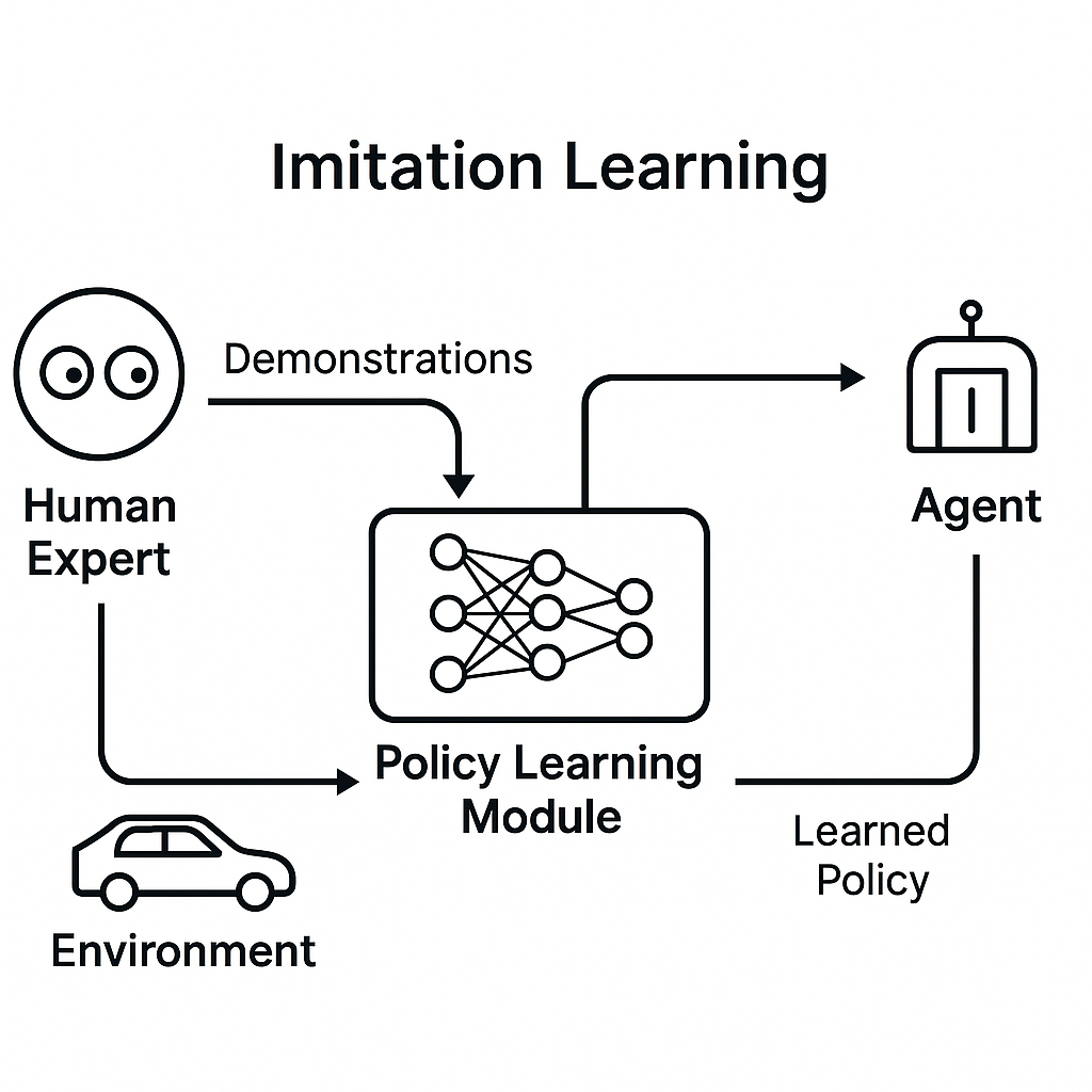
Imitation Learning: A Head Start from Classical Experts
Before unleashing our agent into the wild, we give it a head start: training it to imitate an expert policy (like LOOK). This is called imitation learning.
Instead of exploring randomly from scratch (which leads to chaotic and unproductive behavior early on), the agent learns to mimic the decisions of a classical policy. It sees state-action pairs from the expert and learns to replicate them by minimizing classification loss.
This stage is surprisingly effective. With a good enough teacher (in our case, LOOK), the agent can learn near-optimal routing behavior even before seeing any rewards.
From the imitation phase, we track model performance by monitoring the total episode reward:
Imitation training loop
# Get actions from the expert (LOOK policy)
with torch.no_grad():
    expert_actions = expert.act(batch_obs)

# Predict actions using the student policy
logits, _ = student.forward(batch_obs)
student_actions = logits.argmax(dim=-1)

# Compute imitation loss
loss = F.cross_entropy(logits, expert_actions)

# Update student policy
optimizer.zero_grad()
loss.backward()
optimizer.step()
Once the agent’s imitation loss drops below a threshold (e.g. 0.2), we switch to PPO and let the agent fine-tune its policy based on actual reward.
The result is a model that starts smart - and gets smarter.
Step 4: Running Experiments
Once the agents are in place - from the deterministic rule-followers to the neural policy explorers - it’s time to test them. All experiments are run using a shared evaluation pipeline built around two key scripts: simulation.run and simulation.evaluate.
-
simulation.runis used to run a single simulation and observe visually how the agent is behaving in a single episode. -
simulation.evaluatebenchmarks trained agents (or classical policies) across fixed workloads to collect consistent performance metrics. It runssimulation.runnum_episodestimes, measuring, total reward and other statistics (e.g. average wait time, travel time, requests served, and runtime duration). This is the script we are going to use to evaluate our agents. This is how it looks like:
These abstractions allow us to plug in different agents, scenarios, and seeds, and output a unified set of stats: total reward, average wait time, travel time, requests served, and runtime duration.
For reproducibility and comparability, each model is evaluated over 1000 episodes on a random workload scenario with default parameters (uniform floor distributions and standard spawn probability).
# My parameters
num_floors = 10
num_elevators = 1
elevator_capacities = 10
max_episode_length = 1000
embedding_dim = 16
hidden_dim = 256
num_layers = 3
use_dropout = True
dropout_prob = 0.1
use_batch_norm = True
num_episodes = 10000
batch_size = 32
value_loss_coef = 0.1
gamma = 0.99
learning_rate = 3e-4
early_stop_loss = 0.000
eval_every = 25
eval_episodes = 10
save_every = 100
Results
After training and evaluation, we compared the performance of various elevator agents - from classic rule-based heuristics to our imitation-trained and PPO-fine-tuned RL models. Each was tested over 1000 episodes using the same random workload scenario with default parameters (uniform floor distribution, fixed spawn probability).
Here’s a summary of the results:
| Agent | Reward (min / mean / max) | Std. Dev. | Wait Time | Travel Time | Requests Served | Avg. Run Duration (s) |
|---|---|---|---|---|---|---|
| FCFS | -3260.21 / -204.63 / 430.82 | 905.86 | 16.33 | 10.82 | 149.76 | 0.17 |
| SCAN | -2197.31 / 402.73 / 492.52 | 108.74 | 11.79 | 7.45 | 195.67 | 0.15 |
| LOOK | -1546.42 / 413.51 / 512.16 | 121.87 | 9.89 | 6.47 | 196.40 | 0.18 |
| Imitation Learning (LOOK) | -1258.86 / 400.98 / 504.51 | 94.89 | 11.42 | 7.66 | 195.81 | 1.49 |
| RL (Imitation + PPO) | -2169.88 / 402.35 / 500.48 | 106.49 | 11.35 | 7.49 | 196.00 | 3.11 |
Why did RL (almost) work - But not quite?
Our imitation learner, trained on LOOK data, performs quite well but noticeably worse than its teacher in aggregate metrics like requests served and average reward. Its larger standard deviation suggests greater policy instability—likely due to its overfitting to specific decision patterns or failing to generalize under noisy traffic.
Our PPO fine-tuned RL model recovers strong performance, nearly matching LOOK in mean reward. This validates RL’s potential to discover long-term policies on its own. However, it still lags slightly in stability and hasn’t yet overtaken the classical baseline in total service quality.
Training RL from scratch remains fragile and sensitive to design decisions, but we’re getting closer. With the right architecture, things might just click.
Conclusion and Takeaways
So… what should the elevator do?
Turns out, even in a simple single-elevator system, that question is far from trivial. We’ve seen how classic algorithms like SCAN and LOOK offer robust, time-tested strategies. They’re not optimal - but they’re predictable, efficient, and surprisingly hard to beat.
Reinforcement learning, while promising, hasn’t quite outperformed the classics yet. But it’s shown signs of potential:
- With imitation learning, we were able to replicate strong heuristics with decent generalization.
- With PPO, we caught a glimpse of long-term learning - but also its fragility in noisy, sparse, real-time environments.
Along the way, we built a fully modular simulation engine, capable of modeling elevators, workloads, and decision agents - all of which can be reused, extended, and challenged by future experiments.
Key Takeaways
- Modeling the problem matters: The quality of your simulation, state space, and reward signals defines the ceiling of what any RL method can learn.
- Classic baselines are strong: LOOK may seem simple, but it encodes decades of engineering wisdom. Use it as a teacher, not just a competitor.
- RL needs structure: Naive MLPs and reward shaping only get you so far. Smart architecture matters.
- Training RL on elevators is fun: And watching a neural agent discover floor-serving etiquette is its own reward.
What’s Next?
In a future Part 2, we’re doubling down on complexity:
- Introducing multi-elevator settings, where coordination becomes key,
- Designing locality-aware neural networks that better encode spatial structure,
- And experimenting with action embeddings, STOP modeling, and smarter exploration.
We’ll try to fix what PPO got wrong - not by making it deeper, but by making it think closer to the problem.
> Because sometimes, the best elevator isn’t the smartest one. It’s just the one that knows when to stop.
References
-
Peters, R. D. (2014). Elevator Dispatching. Elevator Technology 9, IAEE: Overview of heuristic and AI-based elevator dispatch algorithms. ↩ ↩2
-
Wikipedia. Elevator Algorithm (SCAN disk scheduling). (link): Explanation of SCAN and LOOK disk scheduling algorithms and their analogy to elevator logic. ↩
-
DiVA Thesis (2015). Scheduling of Modern Elevators: Technical discussion of nearest-car heuristics and “figure of suitability” scoring in dispatch systems. ↩
-
Elevator Wiki. Destination Dispatch, Peak Period Control (1937). (link): Historical and technical overview of destination-based scheduling and group control modes. ↩
-
Crites, R. & Barto, A. (1996). Improving Elevator Performance Using Reinforcement Learning. NeurIPS: Early application of multi-agent RL to elevator group control, (link) ↩ ↩2
-
ZIB Report (2005). Online Optimization of Multi-Elevator Systems: Notes on MILP and NP-hardness of elevator scheduling. ↩ ↩2